Build a spectrum analyser with Scroll pHAT and pHAT DAC

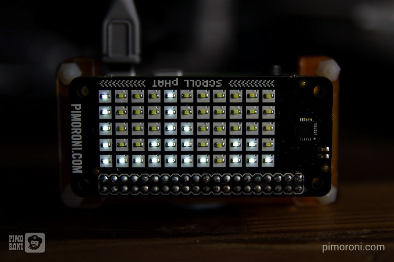
This tutorial will show you how to set up a tiny little spectrum analyser with a Raspberry Pi Zero, a pHAT DAC (digital to analogue converter) and a Scroll pHAT LED matrix. We'll walk through how to solder the pHATs, how to install the necessary software and then how the code itself works.
What you'll need:
- A Raspberry Pi Zero
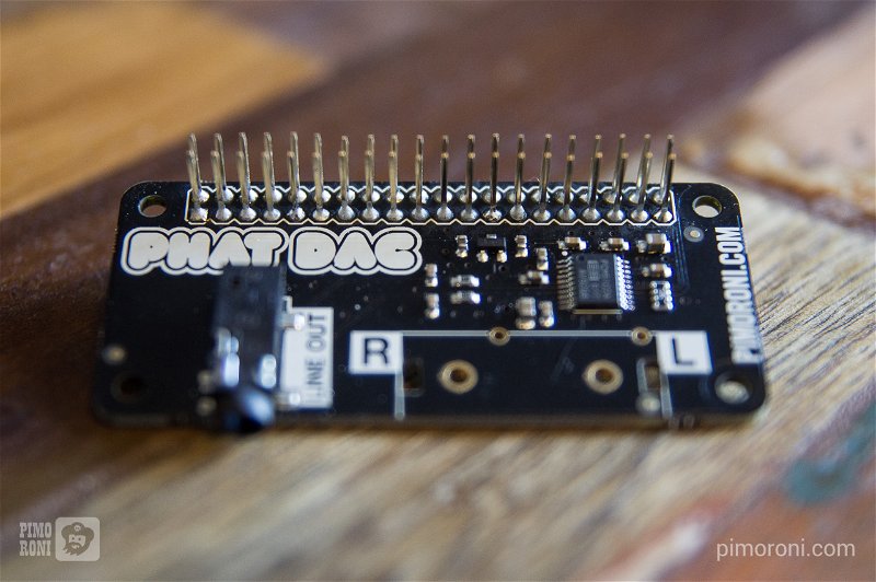
- A pHAT DAC
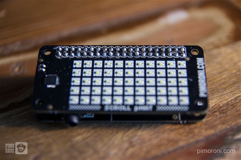
- A Scroll pHAT
- A male 40 pin header
- An extended female 40 pin header
- A soldering iron with a conical/pointed tip
- Lead-free solder
- A roll of masking tape (recommended, but not essential)
- Panavise (recommended, but not essential)
Soldering the Pi Zero and pHATs
Since the Pi Zero and the pHAT come un-soldered, you'll need to solder headers onto them first. We've written a little guide to show you how to solder headers onto pHATs, so we'd suggest that you refer to that if you're not already a dab hand with a soldering iron.
First, you'll want to solder a male 40 pin header onto the Pi Zero. Make sure that you solder it so that the longer ends of the pins are pointing up the way, and the shorter ends are protruding down through the holes on the Pi Zero where you'll solder them.
The pHATs will need to be stacked on top of each other, with the pHAT DAC below and the Scroll pHAT on top. There are a couple of ways to do this.
If you want to use the Scroll pHAT for other things besides just this spectrum analyser, then you can just solder a normal 40 pin female header to it and solder an extended 40 pin female header to the pHAT DAC, meaning that you can mount the Scroll pHAT on the pHAT DAC in the usual way.
Or, you can do it more permanently by first soldering the extended female header to the pHAT DAC and then soldering the Scroll pHAT directly on top and clipping any extra bits of pin protruding out from the top afterwards.
We chose to do it the permanent way, with the extended female header, and you can see the two stages in the images below.


Setting up pHAT DAC
Make sure that you're starting with a fresh, up-to-date version of Raspbian, as this is what was used when putting together this tutorial and we can't vouch that it will work properly otherwise.
There's a handy one line installer for pHAT DAC that should get everything set up properly. In the terminal, type the following:
curl https://get.pimoroni.com/phatdac | bash
The installer should prompt you to reboot but, if it doesn't, type in the
terminal, sudo reboot.
You can test that it has worked properly by connecting a speaker to your pHAT DAC (make sure that you don't use headphones, as pHAT DAC is designed for line level output) and typing:
aplay /usr/share/sounds/alsa/Front_Center.wav
We also need to install the alsaaudio Python library. Do this by typing:
sudo apt-get install python-alsaaudio
Assuming that all worked, we'll move on to getting Scroll pHAT installed and working.
Setting up Scroll pHAT
There's also a one line installer for Scroll pHAT. Type the following in the terminal to install the Scroll pHAT library:
curl https://get.pimoroni.com/scrollphat | bash
Again, it should prompt you to reboot but, if it doesn't, type sudo reboot in
the terminal.
You can test that it worked by typing, in the terminal:
sudo python scroll-phat/examples/cpu.py
This should graph out your CPU usage, scrolling from right to left.
Fast Fourier Transform (FFT)
The Fast Fourier Transform is an incredibly nifty way of converting values from the time domain into a spectrum of different frequencies for a given time period. In this way, we can average out, or compress, audio data in real time. The niftiest feature of FFT is how quick an algorithm it is for the amount of data processed. It's used commonly in image, video and audio compression, and you're probably taking advantage of it many times each day without even being aware of it.
Fortunately, there's a Python library, Numpy, that can do FFT, amongst many other things.
We can read in audio data in real time, use the FFT at a given sampling rate to compute the FFT for the whole audio spectrum, and then average it out into the number of bands we want - 11 - to fit onto Scroll pHAT's matrix.
The code
Imports
We'll do all of this in Python. We'd recommend that you put all of the
following code into a text file, in your favourite text editor, and then
save it as something like spectrum_analyser.py. Of course, you could do it
all interactively in a Python prompt, but that'd be a real pain.
Once your code is complete, you can open a terminal and run your code by typing
sudo python spectrum_analyser.py.
First, we'll import all of the libraries that we need for our little spectrum analyser program:
import sys
import wave
import alsaaudio as aa
from struct import unpack
import numpy as np
import scrollphat
We'll need the sys library to parse the command line arguments passed to our
script.
The wave, alsaaudio, struct and numpy libraries will be used to read in and
analyse the audio we pass to our program.
Finally, we'll use the scrollphat library to display the audio data on our
Scroll pHAT matrix.
Settings
Below our imports, and before our functions, we'll set some settings that will determine how our audio is processed.
First, we'll open our .wav file, using the wave library, having grabbed the
filename with sys.argv[1] from the sys library:
wavfile = wave.open(sys.argv[1], 'r')
Passing the filename as an argument is a better approach than hard-coding the
path to the file, as we can change what file we pass on the fly. To run our
program with a .wav file called sailorshornpipe.wav we'd type the following
in the terminal once our code is complete:
sudo python spectrum_analyser.py sailorshornpipe.wav
Note that it's sys.argv[1] rather than sys.argv[0], because sys.argv[0]
refers to the program name itself.
Next, we'll set some parameters for the audio output. As well as processing the audio, we need to feed the audio back out, so that we can hear it as well as seeing it!
sample_rate = wavfile.getframerate()
no_channels = wavfile.getnchannels()
chunk = 4096

output = aa.PCM(aa.PCM_PLAYBACK, aa.PCM_NORMAL)
output.setchannels(no_channels)
output.setrate(sample_rate)
output.setformat(aa.PCM_FORMAT_S16_LE)
output.setperiodsize(chunk)
We get the sample rate and number of channels from our .wav file, and set the
chunk size, which determines how many chunks our audio is broken into for
processing.
Then, we set up an alsa audio output and set the same parameters that we got
from our .wav file.
We'll need a couple of lists in which to store our values that we get from the audio, and also a list of weightings that will be applied to each of our frequency bands.
matrix    = [0, 0, 0, 0, 0, 0, 0, 0, 0, 0, 0]
power     = []
weighting = [1, 1, 2, 4, 8, 8, 8, 8, 16, 16, 16]
The power list will store values from our Fourier transform and the matrix
list will store the actual values that we'll display on our spectrum. Because
different frequency bands will be more prevalent than others, we weight each
band differently, to even out the spectrum. This is what our weighting list
does, and you can tweak these values if you like, to get your spectrum looking
the way you want. These values worked well for us.
Lastly, we set the brightness of our Scroll pHAT a little below full brightness.
scrollphat.set_brightness(5)
The Fast Fourier Transform
We'll write two different functions to help with our Fast Fourier Transform.
The first is a simple function that takes a frequency value and returns its index (position) in our array of computed FFT values. This will allow us to average out each frequency band when we compute the FFT values.
def power_index(val):
    return int(2 * chunk * val / sample_rate)
The second is the function that will compute the FFT for each chunk of our audio data. Here's the complete function, and then we'll break it down step-by-step.
def compute_fft(data, chunk, sample_rate):
    global matrix
    data = unpack("%dh" % (len(data) / 2), data)
    data = np.array(data, dtype='h')

    fourier = np.fft.rfft(data)
    fourier = np.delete(fourier, len(fourier) - 1)

    power = np.abs(fourier)

    matrix[0] = int(np.mean(power[power_index(0)    :power_index(156) :1]))
    matrix[1] = int(np.mean(power[power_index(156)  :power_index(313) :1]))
    matrix[2] = int(np.mean(power[power_index(313)  :power_index(625) :1]))
    matrix[3] = int(np.mean(power[power_index(625)  :power_index(1000) :1]))
    matrix[4] = int(np.mean(power[power_index(1000) :power_index(2000) :1]))
    matrix[5] = int(np.mean(power[power_index(2000) :power_index(3000) :1]))
    matrix[6] = int(np.mean(power[power_index(3000) :power_index(4000) :1]))
    matrix[7] = int(np.mean(power[power_index(4000) :power_index(5000) :1]))
    matrix[8] = int(np.mean(power[power_index(5000) :power_index(6000) :1]))
    matrix[9] = int(np.mean(power[power_index(6000) :power_index(7000) :1]))
    matrix[10] = int(np.mean(power[power_index(7000):power_index(8000) :1]))

    matrix = np.divide(np.multiply(matrix, weighting), 1000000)
    matrix = matrix.clip(0, 5)
    matrix = [float(m) for m in matrix]

    return matrix
We pass a number of different things into the function: the piece of audio data itself, the chunk size and the sample_rate.
compute_fft(data, chunk, sample_rate)
Next, we declare matrix as a global variable, meaning that it exists outside
the scope of this function.
We also unpack the binary C short type data to a type that Python can interpret
and then convert it into a numpy array, ensuring that we tell it that the data
is in the C short type - dtype='h'.
global matrix
data = unpack("%dh" % (len(data) / 2), data)
data = np.array(data, dtype='h')
Next, we do the actual Fourier transform. We're using the rfft function from
numpy.fft since we're using real data, and then we delete the last element in
the array, so that our array size matches the chunk size.
fourier = np.fft.rfft(data)
fourier = np.delete(fourier, len(fourier) - 1)
Because the Fourier transform will return positive and negative values, we take the absolute values of the numpy array, which converts all of the negative values to positive ones.
power = np.abs(fourier)
We need to split our frequency spectrum up into 11 bands to display on our
Scroll pHAT. To do that, we'll slice our power array of FFT-computed
frequencies into 11 pieces using our power_index function, take the mean
(average) of each piece, and then read them into our matrix list at the
appropriate position.
matrix[0] = int(np.mean(power[power_index(0)    :power_index(156) :1]))
matrix[1] = int(np.mean(power[power_index(156)  :power_index(313) :1]))
matrix[2] = int(np.mean(power[power_index(313)  :power_index(625) :1]))
matrix[3] = int(np.mean(power[power_index(625)  :power_index(1000) :1]))
matrix[4] = int(np.mean(power[power_index(1000) :power_index(2000) :1]))
matrix[5] = int(np.mean(power[power_index(2000) :power_index(3000) :1]))
matrix[6] = int(np.mean(power[power_index(3000) :power_index(4000) :1]))
matrix[7] = int(np.mean(power[power_index(4000) :power_index(5000) :1]))
matrix[8] = int(np.mean(power[power_index(5000) :power_index(6000) :1]))
matrix[9] = int(np.mean(power[power_index(6000) :power_index(7000) :1]))
matrix[10] = int(np.mean(power[power_index(7000):power_index(8000) :1]))
Lastly, we multiply our matrix by our weighting list and divide by 1,000,000 to
get the numbers into a more sensible scale. We'll also clip each of the 11
values to a maximum of 5, so that they can be displayed on Scroll pHAT's
columns, which are 5 LEDs high, and then convert them to floats to make them
play nice with Scoll pHAT's graph method.
matrix = np.divide(np.multiply(matrix, weighting), 1000000)
matrix = matrix.clip(0, 5)
matrix = [float(m) for m in matrix]
Processing the audio
Our wavfile, read in with the wave library, has a convenient readframes
method that can read the audio data in chunks of a given size. We can simply
use our chunk variable that we set earlier to tell it how big the chunks
should be. Each time this function is called, it will parse another chunk of
audio. Ideal for our purposes!
data = wavfile.readframes(chunk)
Finally, we use a while loop to i) output the audio, ii) compute the FFT,
iii) display the FFT bands on Scroll pHAT with its graph method, specifying
the range (0-5) and, iv) to read the next chunk of data.
while data != '':
    output.write(data)
    matrix = compute_fft(data, chunk, sample_rate)
    scrollphat.graph(matrix, 0, 5)
    data = wavfile.readframes(chunk)
Running the example
As we mentioned above, you can run the example on your wav audio file by
typing the following in a terminal, assuming your audio file is called
sailorshornpipe.wav.
sudo python spectrum_analyser.py sailorshornpipe.wav
Here's an example of how it should look.

In theory, it's possible to stream audio data directly into a Python script, so you could stream all of the system audio through the script and display the spectra on Scroll pHAT, although that's beyond the scope of this tutorial. We'd encourage you to give it a shot though.
There's a complete copy of the code below.
import sys
import wave
import alsaaudio as aa
from struct import unpack
import numpy as np
import scrollphat

wavfile = wave.open(sys.argv[1], 'r')

sample_rate = wavfile.getframerate()
no_channels = wavfile.getnchannels()
chunk = 4096

output = aa.PCM(aa.PCM_PLAYBACK, aa.PCM_NORMAL)
output.setchannels(no_channels)
output.setrate(sample_rate)
output.setformat(aa.PCM_FORMAT_S16_LE)
output.setperiodsize(chunk)

matrix    = [0, 0, 0, 0, 0, 0, 0, 0, 0, 0, 0]
power     = []
weighting = [1, 1, 2, 4, 8, 8, 8, 8, 16, 16, 16]

scrollphat.set_brightness(5)
def power_index(val):
    return int(2 * chunk * val / sample_rate)

def compute_fft(data, chunk, sample_rate):
    global matrix
    data = unpack("%dh" % (len(data) / 2), data)
    data = np.array(data, dtype='h')

    fourier = np.fft.rfft(data)
    fourier = np.delete(fourier, len(fourier) - 1)

    power = np.abs(fourier)
    matrix[0] = int(np.mean(power[power_index(0)    :power_index(156) :1]))
    matrix[1] = int(np.mean(power[power_index(156)  :power_index(313) :1]))
    matrix[2] = int(np.mean(power[power_index(313)  :power_index(625) :1]))
    matrix[3] = int(np.mean(power[power_index(625)  :power_index(1000) :1]))
    matrix[4] = int(np.mean(power[power_index(1000) :power_index(2000) :1]))
    matrix[5] = int(np.mean(power[power_index(2000) :power_index(3000) :1]))
    matrix[6] = int(np.mean(power[power_index(3000) :power_index(4000) :1]))
    matrix[7] = int(np.mean(power[power_index(4000) :power_index(5000) :1]))
    matrix[8] = int(np.mean(power[power_index(5000) :power_index(6000) :1]))
    matrix[9] = int(np.mean(power[power_index(6000) :power_index(7000) :1]))
    matrix[10] = int(np.mean(power[power_index(7000):power_index(8000) :1]))

    matrix = np.divide(np.multiply(matrix, weighting), 1000000)
    matrix = matrix.clip(0, 5)
    matrix = [float(m) for m in matrix]

    return matrix

data = wavfile.readframes(chunk)

while data != '':
    output.write(data)
    matrix = compute_fft(data, chunk, sample_rate)
    scrollphat.graph(matrix, 0, 5)
    data = wavfile.readframes(chunk)
Search above to find more great tutorials and guides.